Checkpoint Champion – Predicting Winners at 25

Authors:

• Xingzhi Cui (tigercui@umich.edu)
• Yun Jong Na (kevinyjn@umich.edu)

---

Table of Contents

1. Introduction
2. Data Cleaning and Exploratory Data Analysis
3. Framing a Prediction Problem
4. Baseline Model
5. Testing for Potential Improvement
6. Model Comparison and Final Selection

---

Spoiler Alert! 🎲

Try the model yourself first!

Read on to see how we built the model!

Introduction

In this project, we explore whether in-game features at the 25 minute cutoff can accurately predict the outcome (win/loss) of League of Legends matches. Our full dataset consists of approximately 9800 matches in 2024 sourced from OraclesElixir, which is a public dataset under Riot Games, containing information on champion selections, team compositions, player roles, and match metadata.

• Central Question: Can a classification model leverage in-game kills, gold, experience information at the 25 minute checkpoint to predict the game result? If so, what predictor is the most influential?
• Motivation: Predictive insights can inform esports strategy and enhance spectator engagement by offering data-driven match forecasts.
• Dataset Details:
  • Rows: 117600, 2 rows per game
  • Relavant Features:
    • gameid: A unique identifier for each game
    • goldat25: Team’s total gold collected by minute 25
    • xpat25: Team’s total experience points gained by minute 25
    • csat25: Team’s total creep score (minion kills) by minute 25
    • killsat25: Total kills achieved by the team by minute 25
    • assistsat25: Total assists by the team by minute 25
    • deathsat25: Total deaths suffered by the team by minute 25
    • opp_goldat25: Opponent team’s total gold collected by minute 25
    • opp_xpat25: Opponent team’s total experience points gained by minute 25
    • opp_csat25: Opponent team’s total creep score by minute 25
    • opp_killsat25: Total kills achieved by the opponent team by minute 25
    • opp_assistsat25: Total assists by the opponent team by minute 25
    • opp_deathsat25: Total deaths suffered by the opponent team by minute 25
    • golddiffat25: Gold difference at minute 25 (goldat25 – opp_goldat25)
    • xpdiffat25: Experience difference at minute 25 (xpat25 – opp_xpat25)
    • csdiffat25: Creep score difference at minute 25 (csat25 – opp_csat25)
    • side: Team side designation (Blue or Red), which can influence draft priority and map control
    • gamelength: Total duration of the match, in seconds, capturing overall game pace
    • league: Regional league or tournament in which the match was played (e.g., LCK, LPL, LEC)

  • Target Variable: result (win = 1, loss = 0)

  • Relevance: Accurate prediction models support coaches and analysts in optimizing in‑game decisions and contribute to the broader field of sports analytics.

---

Data Cleaning and Exploratory Data Analysis

1. Row Selection
   • Level filter: From the original 12 rows per match, keep only the two team‑level records (data = data[data['position'] == 'team']); discard all player‑level entries.
2. Feature Selection
   • Restricted to features measured at 25 minutes.
   • Removed time‑static variables (e.g. total dragons slain).
   • Dropped perfectly collinear stats (ex: killsAs25 vs. opp_deathsAt25) to aid interpretability.
3. Imputation Strategies and Missing‑Value Handling
   • Assessment of missingness: We found that rows lacking any 25‑minute metric (gold, kills, objectives, etc.) account for roughly 46.58% of our team‑level data.
   • Rationale for dropping: A missing 25‑minute value indicates that the game state wasn’t recorded at that cut‑off, so these rows contain no usable mid‑game information. Imputing them would introduce unfounded assumptions, so we removed all records with missing 25‑minute features. ​Below is a visualization of the row count comparison before and after dropping missing values.
   • Filling in Missing Values If one of the values was missing in the 25 minute metrics, all the other values for the 25 minute features were missing as well. We did not fill in missing values, instead we removed the entire rows.

Head of Cleaned Data With Relevant Columns:

gameid	result	goldat25	xpat25	csat25	opp_goldat25	opp_xpat25	opp_csat25	golddiffat25	xpdiffat25	csdiffat25	killsat25	assistsat25	deathsat25	opp_killsat25	opp_assistsat25	opp_deathsat25	side	gamelength	league
LOLTMNT99_132542	1	52523	58329	831	39782	47502	752	12741	10827	79	20	47	7	7	14	20	Blue	1446	TSC
LOLTMNT99_132542	0	39782	47502	752	52523	58329	831	-12741	-10827	-79	7	14	20	20	47	7	Red	1446	TSC
LOLTMNT99_132665	1	45691	55221	850	44232	51828	825	1459	3393	25	17	28	11	11	15	17	Blue	2122	TSC
LOLTMNT99_132665	0	44232	51828	825	45691	55221	850	-1459	-3393	-25	11	15	17	17	28	11	Red	2122	TSC
LOLTMNT99_132755	1	43051	53899	822	41959	51633	854	1092	2266	-32	10	19	7	7	11	10	Blue	2099	TSC

Univariate Analysis The histogram shows the distribution of gold difference at 25 minutes, calculated as a team’s gold minus their opponent’s. As expected, the distribution is perfectly symmetrical around zero, since one team’s gain is the other’s loss. This confirms that the feature captures relative advantage, which indicates how much more or less gold a team has compared to their opponent. Relative advantage is a key factor in predicting match outcomes. A value above zero means the team is ahead; below zero means they’re behind. Since golddiffat25 directly reflects in-game dominance, it serves as a highly informative predictor. While most games are fairly balanced (clustered near 0), the long tails represent matches where one team gains a significant economic lead, which often correlates with winning. The histogram for distribution of team gold at 25 minutes showcases how most teams cluster around 42k ~ 42.999k gold, indicating the consistent game pacing across matches.

Bivariate Analyses and Aggregations The boxplot compares the gold difference at the 25 minute mark between winning and losing teams. Winning teams consistently showed a strong positive gold difference, while the losing teams often fell behind. The side by side visualization highlights the predictive power of this single feature: the teams leading in gold at minute 25 have a significant competitive advantage and are more likely to win the game match. Thus, economic leads are strongly associated with successful match outcomes. The boxplot for kills at 25 minutes vs results showcases that the teams with more kills at the 25 minute mark are more likely to win, demonstrating the importance of kills. The boxplot for kills at 25 minutes vs gold at 25 minutes reveal the positive relationship between kills and gold at 25 minutes, and we see clusters of winners towards the upper right. This reinforces how kills often translate to stronger economies at match wins.

The aggregate table below presents the average values of critical mid-game performance metrics at 25 minutes, grouped by match outcome. Winning teams (result = 1) consistently outperform the losing teams (result = 0) in every key statistic: gold, experience, creep scores, kills, whil also resulting in less deaths. These patterns validate that mid game performance strongly correlates with success, highlighting the predictive value of these features for the classification model.

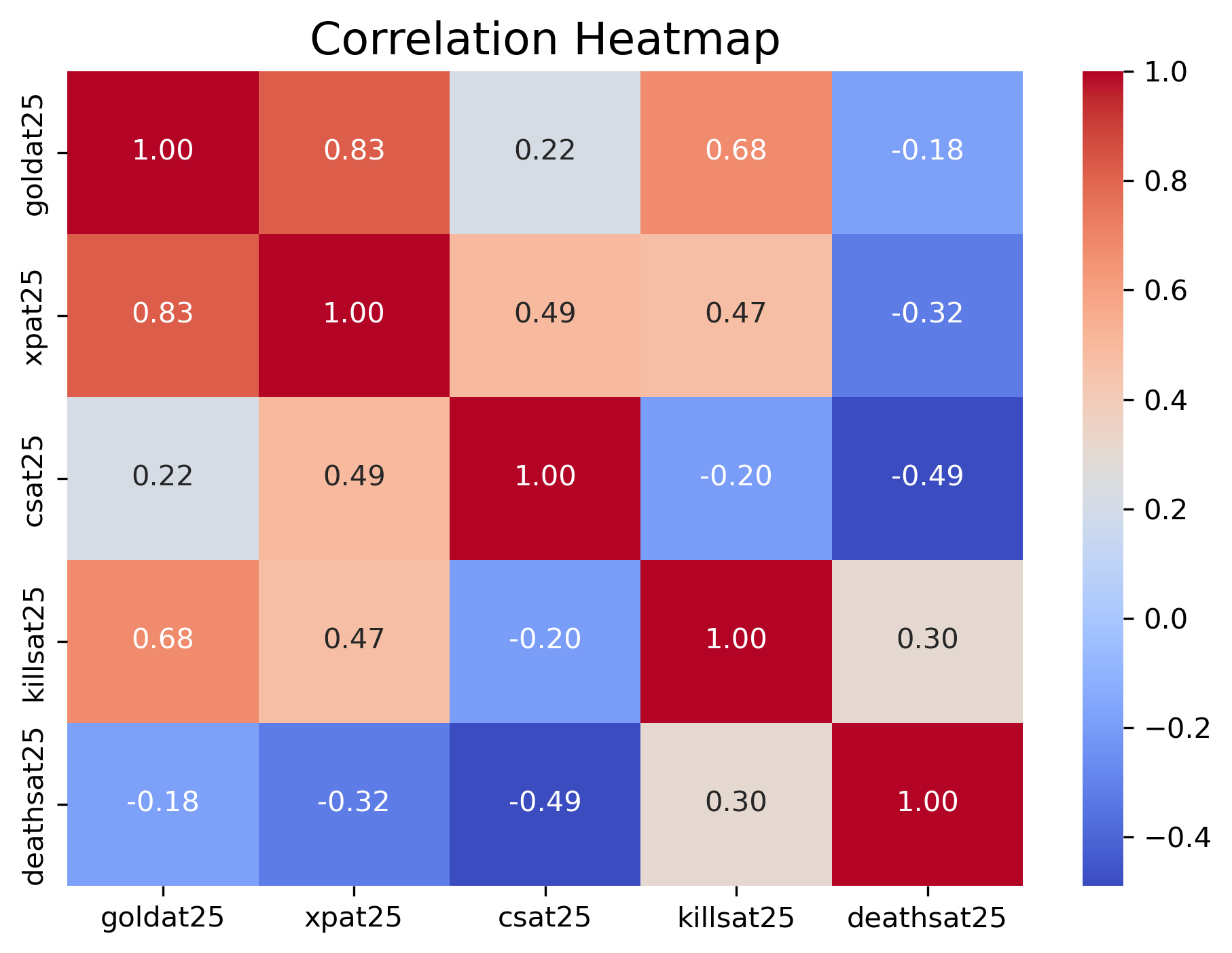
Issues with Multicollinearity

Even after dropping the most obvious redundancies, many of our 25‑minute features remain highly correlated. For example, teams that secure more kills typically accumulate more gold and experience, while opponents with higher death counts correspondingly lag behind. This interdependence can lead to unstable coefficient estimates in a standard logistic regression. Therefore, in the following regression models, we will need to either address these issues or interpret the results with caution.

Framing a Prediction Problem

• Task: Binary classification of match outcome, result (1 = win, 0 = loss).
• Features: All in‑game metrics available at the 25 minute mark after the filtering and cleaning steps described in Data Cleaning and Exploratory Data Analysis. We exclude any variables that aren’t known at minute 25 (e.g. final kill totals).
• Evaluation Metric: Accuracy, defined as the proportion of correct predictions: 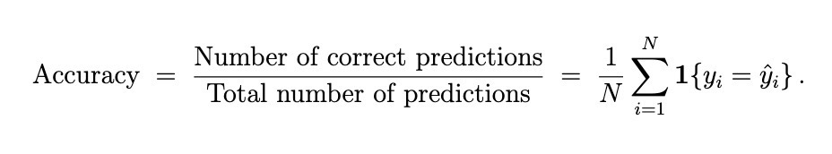where yi is the true label and yi hat is the model’s prediction.
• Prediction Question:

  What game performance metric at the 25 minute checkpoint is the most influential to the outcome of the match?

Baseline Model

To establish a performance benchmark, we trained a simple logistic regression on our 25‑minute features for the team, exluding the information of their opponents.

Data Partitioning
We split the cleaned dataset into training (70%) and test (30%) sets, preserving the win/loss balance via stratification.

Baseline Model Information

Data Type	Features	Processing Method
Quantitative	goldat25, xpat25, csat25, killsat25, deathsat25	StandardScaler
Ordinal	–	–
Nominal	–	–

Results Output

Model Name	num_non_zero	training_accuracy	testing_accuracy	ROC_accuracy
Baseline_Simple_Logistic_Regression	5	0.809433	0.812473	0.897624

Model Analysis

The baseline logistic regression achieves 80.94% accuracy on the training set and 81.25% on the test set, with a ROC‑AUC of 0.8976—indicating strong overall discrimination between wins and losses. However, the presence of multicollinearity among mid‑game features, as indicated in Issues with Multicollinearity, suggests that regularized models or dimensionality‑reduction techniques may further improve stability and performance in subsequent modeling steps. Moreover, including more features may improve the predictive power of the model.

Testing for Potential Improvement

-Feature Engineering

To enrich our predictive signal, we extended the feature set as follows:

• Categorical Variables:
  • League and Side were one‑hot encoded via ColumnTransformer + OneHotEncoder to capture structural differences across competitive regions and team assignments.
• Continuous Variables:
  • Game Length was retained as a numeric feature and standardized alongside other in‑game metrics.
• Opponent Metrics:
  • We introduced opp_goldat25, opp_xpat25, and opp_csat25 to account for the opposing team’s mid‑game performance, which can directly influence outcome probabilities.

---

-Addressing Multicollinearity

Our initial OLS‑based logistic regression revealed unstable coefficient estimates under high predictor correlation. Multicollinearity inflates variance, undermines interpretability, and can degrade out‑of‑sample performance.

To mitigate these issues, we evaluate three modeling strategies expressly designed to handle correlated features:

1. Ridge Logistic Regression (L2 Regularization)
   Applies an L2 penalty to shrink coefficient magnitudes, reducing variance without discarding predictors.

2. LASSO Logistic Regression (L1 Regularization)
   Introduces an L1 penalty to drive some coefficients to zero, thus performing automatic variable selection and alleviating redundancy.

3. Recursive Feature Elimination (RFE)
   Recursively removes the least important features based on model performance, yielding a parsimonious set of predictors.

Each approach offers a robust mechanism for stabilizing estimates and improving generalization in the presence of multicollinearity. Subsequent sections detail their implementation and comparative evaluation.

Model Comparison and Final Selection

Model Name	num_non_zero	training_accuracy	testing_accuracy	ROC_accuracy
Baseline_Simple_Logistic_Regression	5	0.809433	0.812473	0.897624
LogisticRegressionCV_L1	9	0.835888	0.8361	0.921376
Ridge_LogisticRegressionCV	57	0.835979	0.836526	0.921788
LogisticRegression_RFECV_BackwardElimination	5	0.835523	0.833972	0.920703

Key Observations:

• The L1‑penalized (LASSO) model matches the highest test accuracy (83.61%) and AUC (0.9214), using only 9 non‑zero coefficients.
• The Ridge model attains similar performance metrics but retains 57 coefficients, increasing complexity and overfitting risk.
• The RFECV approach yields a very sparse model (5 features) but with slightly lower test accuracy (83.40%) and AUC (0.9207).
• The Baseline logistic regression lags behind on both accuracy and discrimination (AUC).

Final Model Choice:
We select the LASSO Logistic Regression as our final model based on its superior balance of performance, sparsity, and stability:

1. Strong performance lift—achieves 83.61% test accuracy (up from 81.25% with the baseline) and ROC‑AUC = 0.9214 (up from 0.8976), nearly matching Ridge’s performance.
2. Controlled complexity—retains only 9 non‑zero coefficients versus 57 in the Ridge model, dramatically reducing overfitting risk.
3. Better than RFECV—outperforms the backward‑elimination approach (5 features, 83.40% accuracy) while still providing a sparse, interpretable solution.
4. Multicollinearity mitigation—automatically zeros out redundant mid‑game metrics, stabilizing coefficient estimates and enhancing generalization.

-Model Properties

Data Type	Features	Processing Method
Quantitative	goldat25, xpat25, csat25, killsat25, deathsat25, opp_goldat25, opp_xpat25, opp_csat25, opp_killsat25, opp_assistsat25, opp_deathsat25, golddiffat25, xpdiffat25, csdiffat25, gamelength, side_binary	StandardScaler
Nominal	league (one‑hot encoded)	OneHotEncoder
Ordinal	–

Model Analysis
The final LASSO logistic regression model retained 9 mid‑game features with non‑zero coefficients:

• goldat25
• xpat25
• csat25
• killsat25
• deathsat25
• opp_goldat25
• opp_xpat25
• opp_csat25
• side_binary

The best hyperparameter (λ) selected is 21.54, corresponding to an inverse‑penalty strength (C = 0.0464). This value was chosen automatically by LogisticRegressionCV, which integrates the regularization‑strength search into its fit routine. By using LogisticRegressionCV rather than a separate GridSearchCV, we leverage solver optimizations (e.g. warm‑starts and efficient coordinate descent for L1) and keep our code concise—no external parameter grid or nested cross‑validation is required, yet we still obtain the optimal penalty for our model.

Interpretation of Model:
These selected predictors underscore the importance of both a team’s own resource accumulation (gold, experience, creep score, kills, deaths) and the opponent’s resource metrics at 25 minutes, as well as map-side assignment (side_binary), in forecasting match outcomes. By zeroing out redundant features, the LASSO model stabilizes coefficient estimates, mitigates multicollinearity, and focuses on the most informative mid‑game indicators—delivering a sparse yet highly discriminative solution.

Interpretation of Feature Coefficients
The final LASSO logistic regression model reveals that:

• goldat25 has the highest positive coefficient, meaning teams with more gold at 25 minutes are significantly more likely to win.

• In contrast, opp_goldat25 and opp_xpat25 have the strongest negative coefficients, indicating that when the opponent has more resources, the chance of winning decreases.

• Other positively weighted features — xpat25, killsat25, and csat25 — emphasize the value of experience, kills, and creep score accumulation.

• deathsat25 contributes negatively, which aligns with intuition: more deaths generally reflect poor team performance.

• Even minor features like side_binary and opp_csat25 show that map side and farming deficits can subtly influence outcomes.

Overall, the model captures the importance of relative mid-game strength — highlighting how both a team’s own performance and their opponent’s stats impact win probability.

Interpretation of Confusion Matrix
The confusion matrix showcases that the final LASSO logistic regression model performs well at distinguishing match outcomes. Out of all test cases:

• 1939 wins were correctly predicted as wins (true positives)

• 1989 losses were correctly predicted as losses (true negatives)

• 398 wins were incorrectly predicted as losses (false negatives)

• 372 losses were incorrectly predicted as wins (false positives)

Overall, the model achieves a balanced and accurate classification of both winning and losing teams, with relatively few misclassifications.